Simple preprocessing

This guide introduces a selection of tools to preprocess the street network, eliminate unwanted gaps, and fix its topology.

import geopandas as gpd
from shapely.geometry import LineString

import neatnet

Close gaps

The first issue that may happen is a disconnected network where The endpoint nodes do not touch. Such a network exhitbits incorrect topology and the results of any graph-based analysis would be wrong. neatnet.close_gaps can fix the issue by snapping nearby endpoints to a midpoint between the two.

l1 = LineString([(1, 0), (2, 1)])
l2 = LineString([(2.1, 1), (3, 2)])
l3 = LineString([(3.1, 2), (4, 0)])
l4 = LineString([(4.1, 0), (5, 0)])
l5 = LineString([(5.1, 0), (6, 0)])

df = gpd.GeoDataFrame(["a", "b", "c", "d", "e"], geometry=[l1, l2, l3, l4, l5])
df.plot(figsize=(10, 10)).set_axis_off()

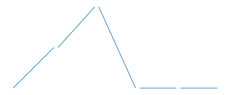
All LineStrings above need to be fixed.

df.geometry = neatnet.close_gaps(df, 0.25)

df.plot(figsize=(10, 10)).set_axis_off()

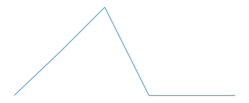
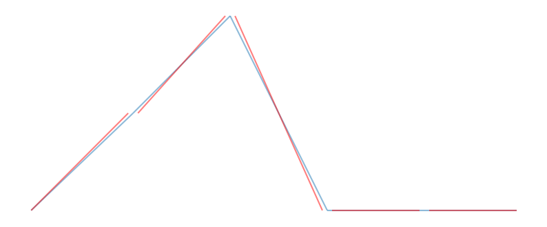
Now we can compare how the fixed network looks compared to the original one.

ax = df.plot(alpha=0.5, figsize=(10, 10))
gpd.GeoDataFrame(geometry=[l1, l2, l3, l4, l5]).plot(ax=ax, color="r", alpha=0.5)
ax.set_axis_off()

Remove interstitial nodes

A very common issue is over-saturated topology. A LineString should end either at street intersections or in dead-ends. However, we often see geometries split randomly along the way, introducing irrelevant nodal data that serves no purpose from a morphological standpoint. neatnet.remove_interstitial_nodes can fix that.

We will use mapclassify.greedy to highlight each segment.

import momepy
from mapclassify import greedy

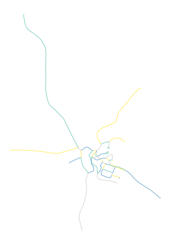
df = gpd.read_file(momepy.datasets.get_path("tests"), layer="broken_network")

df.plot(greedy(df), categorical=True, figsize=(10, 10), cmap="Set3").set_axis_off()

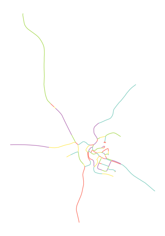
You can see that the topology of the network above is not as it should be.

For a reference, let’s check how many geometries we have now:

len(df)

83

Okay, 83 is a starting value. Now let’s remove interstitial nodes.

fixed = neatnet.remove_interstitial_nodes(df)

fixed.plot(
    greedy(fixed), categorical=True, figsize=(10, 10), cmap="Set3"
).set_axis_off()

From the figure above, it is clear that the network is now topologically correct. How many features are there now?

len(fixed)

56

We have been able to represent the same network using 27 fewer features.

Extend lines

In some cases, we may want to close some gaps by extending existing LineStrings until they meet other geometries.

l1 = LineString([(0, 0), (2, 0)])
l2 = LineString([(2.1, -1), (2.1, 1)])
l3 = LineString([(3.1, 2), (4, 0.1)])
l4 = LineString([(3.5, 0), (5, 0)])
l5 = LineString([(2.2, 0), (3.5, 1)])

df = gpd.GeoDataFrame(["a", "b", "c", "d", "e"], geometry=[l1, l2, l3, l4, l5])
df.plot(figsize=(10, 10)).set_axis_off()

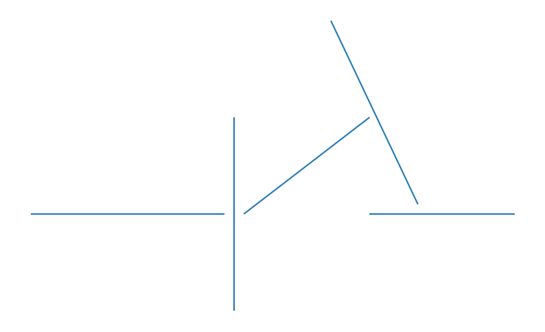
The situation above is typical. The network is almost connected, but there are gaps. Let’s extend geometries and close them. Note that we cannot use neatnet.close_gaps in this situation as we are not snapping endpoints to endpoints.

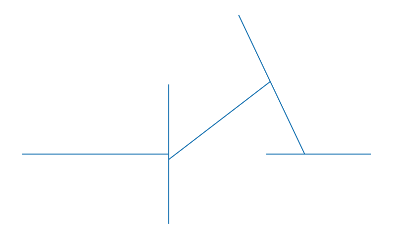
extended = neatnet.extend_lines(df, tolerance=0.2)

extended.plot(figsize=(10, 10)).set_axis_off()

ax = extended.plot(figsize=(10, 10), color="r")
df.plot(ax=ax)
ax.set_axis_off()

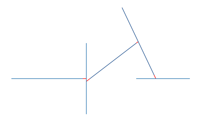
The figures above are self-explanatory. However, remember that the extended network is not topologically correct and is not suitable for network analysis directly. Use induce_nodes to fix it if needed.

For more details and further options, see the API documentation.